Most of what we do day-to-day involves calling LLMs that already exist. But we wanted to know what’s actually happening underneath training, so we spent some time building one from scratch following Andrej Karpathy’s nanoGPT video. The dataset is small (12 Mark Twain books from Project Gutenberg, about 7 megabytes of text). The models are tiny by industry standards. The point was to watch the training behavior with our own eyes on our own hardware, not to produce something extraordinary. This is the first of three posts on that work.
The Setup
Training ran on our NVIDIA DGX Spark, the same workstation we used in the benchmark posts. The model reads text one character at a time, so the “vocabulary” is the 114 unique characters that appear in the Twain corpus (letters, digits, punctuation, whitespace). 90% of the text was used for training, 10% held out for validation.
Two models in this post:
- A bigram model (about 13,000 parameters): given the current character, predict the next one. No memory of anything earlier. The simplest thing that technically counts as a language model.
- A small transformer (about 10.8 million parameters, 830× larger): same task, but with attention. It can look back at the previous 256 characters when predicting the next one.
Both trained for 5,000 iterations on the same data, same split, same random seed.
A note on prompts. Every generated sample shown in this post starts from a single tab character (\t) as the prompt, not a meaningful phrase like “Once upon a time” or “Tom said,”. A tab gives the model a neutral zero-context start, so the output you see is the model freewheeling from nothing rather than reacting to text that might favor a particular dataset or style.
Establishing the Baseline Model – Bigram
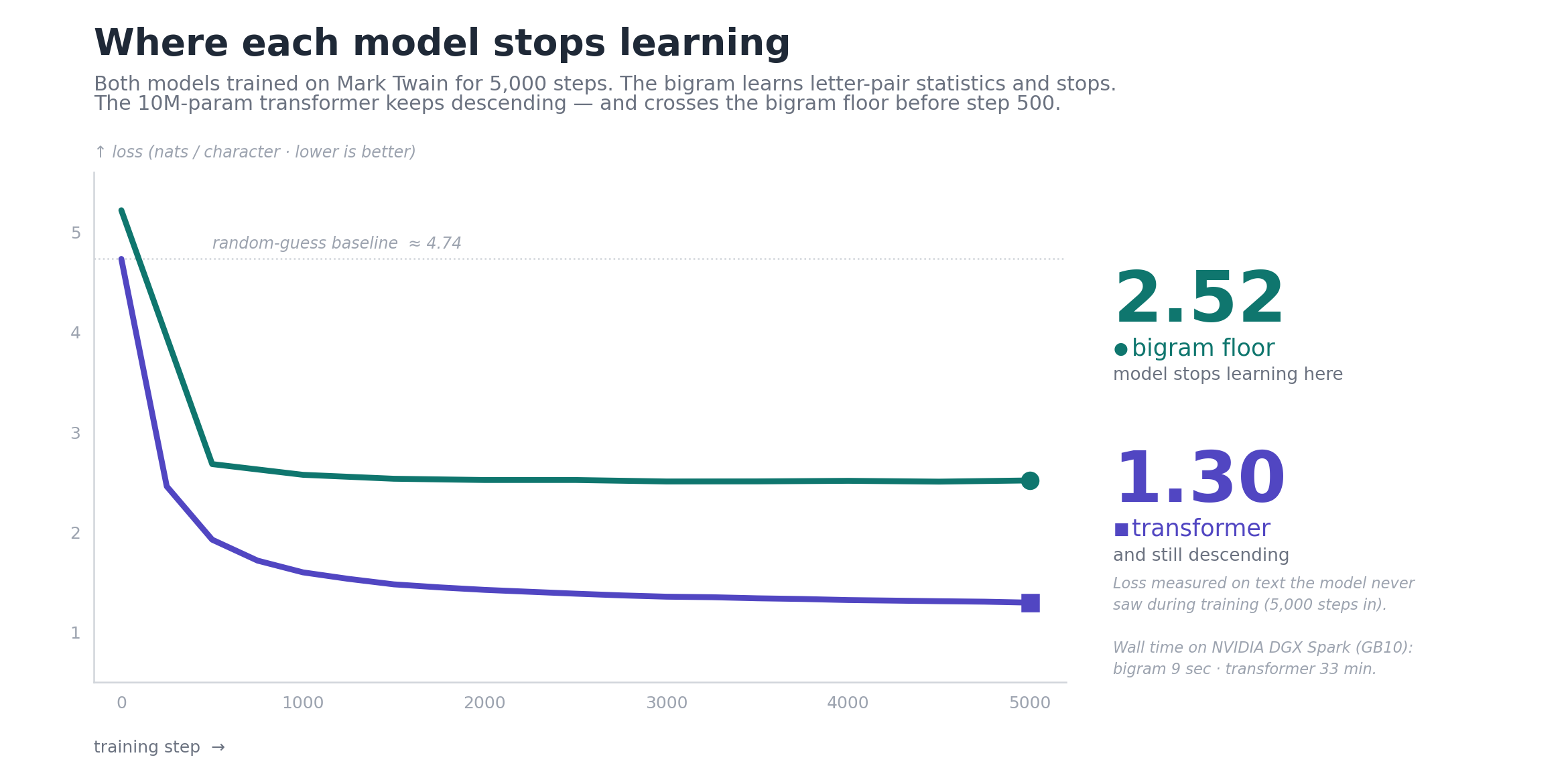
The bigram’s loss dropped from 5.22 to 2.51 in the first 500 iterations and then flatlined. We kept training for another 4,500 iterations and the loss did not change.
The plateau is the model’s ceiling. Bigram models only see one character of context, so once the letter-pair statistics are captured there is nothing else to fit. Generation sample after 5,000 iterations:
“hepecirdus de abrlwhinge m the wh g, Th Ke. izeangeseemaury-t thel the r. u—erig thead_hep MGU tas. hebyt bler arerthe ce iminoolapion tond lad t. icoor us thio ROn imaruly tonf…”
That output is what loss = 2.51 sounds like: letter pairs, a handful of incidental real words, no sentence structure, no meaning. It is the baseline any real model on this dataset has to beat.
Adding Attention
The transformer started at the same loss (4.74, basically ln(114)) and dropped past the bigram’s 2.51 baseline by step 500. By step 5,000 it landed at a training loss of 1.21 and a validation loss of 1.30. The full curves:
Generation sample after 5,000 iterations:
“Vindeberk. Where Saw the week is the dramazy roading over the thick wood. He tranquilled to himself, that would have posted one book washed from a snatch coin, committs selled upon his armed in a grance Ameracharlel’s Track command, who yeaes betheld upon on defect sometimation, very dition of tree, called by his wagon and by fleeb-over his lo dogs…”
Many of the words are real and the made-up ones sound like Twain coinages rather than random letter strings (Vindeberk, tranquilled, Ameracharlel). The output reads as Twain-flavored, even though it is not saying anything coherent.
A Second Dataset
Everything above is one dataset (Twain). The other two posts in this series compare Twain against a second, much larger dataset called TinyStories: about 1.9 billion characters of synthetic children’s stories, roughly 250 times the size of Twain. Where Twain is a slice of one author’s 19th-century prose, TinyStories is a vast pile of formulaic kid-story text (small vocabulary, repetitive sentence templates, lots of “Once upon a time” openers).
Before we use the two datasets to do anything interesting, one calibration is worth locking in: the absolute loss numbers across these two datasets are not directly comparable, because the two corpora have different intrinsic per-character predictability. To show that concretely, we ran the same bigram model on TinyStories. Same architecture, same training budget, same random seed. Only the data changed.
| Dataset | Vocab | Random baseline ln(vocab) | Bigram converged loss |
|---|---|---|---|
| Twain (7.4M chars) | 114 | 4.74 | 2.51 |
| TinyStories (1.9B chars) | 174 | 5.16 | 2.30 |
At the letter-pair level alone, TinyStories text is more predictable than Twain text by 0.21 nats. That holds even though TinyStories has a larger character set (174 vs 114) and therefore has further to descend from random.
TinyStories bigram sample after 5,000 iterations:
“buredallomy t ay fobapomyo to ser ad wandacret tharom’soo y t se Loy. d “Lo andareckethrtousan theande an ef lomy. nd tog hindinerk! bo Juted…”
Reading the two bigram samples side by side, the 0.21-nat gap does not jump out as readability: both still look like gibberish. The numerical floor differs; the qualitative output does not. Letter-pair statistics alone are not enough to produce real words at either floor.
Why this matters for the rest of the series. The next two posts compare loss numbers between models trained on each dataset, and the intuitive reading of “TinyStories loss 0.73, Twain loss 1.21, therefore the TinyStories model is better” is wrong. The loss gap between datasets is already present at the bigram baseline, before any sophisticated model gets involved. Within a dataset, comparing model A to model B is meaningful. Across datasets, the only meaningful comparison is the shape of the train-vs-val divergence, which is what the next post turns on.
What We’re Not Concluding
This covers two datasets, one tokenization (character-level), and two model classes (a bigram baseline and a small transformer). The transformer sample is what character-level training on 7 megabytes of Twain produces; a different dataset or a larger model produces visibly different prose, which is the subject of the next two posts. We are not making general claims about how language models work from this one run. The point was to give the team a concrete visual for how training actually behaves at the simplest scale, and to set up the cross-dataset comparison that the rest of the series builds on.